In the first blogpost we have provided a dataset containing side-channel measurements of a protected AES implementation using masking and shuffling countermeasures. For more details about the dataset and the way it was generated, please refer to the notebook on our gitlab repository. It explains where the points of leakage are, and how the operation shuffling was made.

This blogpost is an extract of a Notebook where we attack the masked and suffled dataset following these steps:

• Classical approach: second-order CPA attack on all SubBytes.
• Refining the CPA through points-of-interest (PoI) averaging.
• Applying Scatter and Spatial Dependency Analysis

Recall on the dataset

import scared
import estraces
import numpy as np
import matplotlib.pyplot as plt

# Get the dataset from disk
ths_disk = estraces.read_ths_from_ets_file('./Nucleo_AES_masked_shuffled.ets')

# The dataset is small enough to be fully loaded into RAM
ths = estraces.read_ths_from_ram(samples=ths_disk.samples[:],
                                plaintext=ths_disk.plaintext[:],
                                key=ths_disk.key[:],
                                mask=ths_disk.mask[:],
                                ciphertext=ths_disk.ciphertext[:])


In this dataset, clock cycles are perfectly aligned with each other, and the jitter is limited to very few samples.

We can display an average trace and highlight 3 main areas:

# Define the identified frames
frames = {'mask': np.arange(0, 100),
         'avg_SubBytes': np.arange(100, 200),
         'all_SubBytes': np.arange(200,1400)}

# Averaging 1000 traces
plt.plot(ths.samples[:1000].mean(0))

plt.axvspan(0, 100, alpha=0.2, facecolor='C0', label='Masks leakage')
plt.axvspan(100, 200, alpha=0.2, facecolor='C1', label='Averaged SubBytes patterns')
plt.axvspan(200, 1400, alpha=0.2, facecolor='C2', label='SubBytes Shiftrow area')

plt.legend()
plt.show()


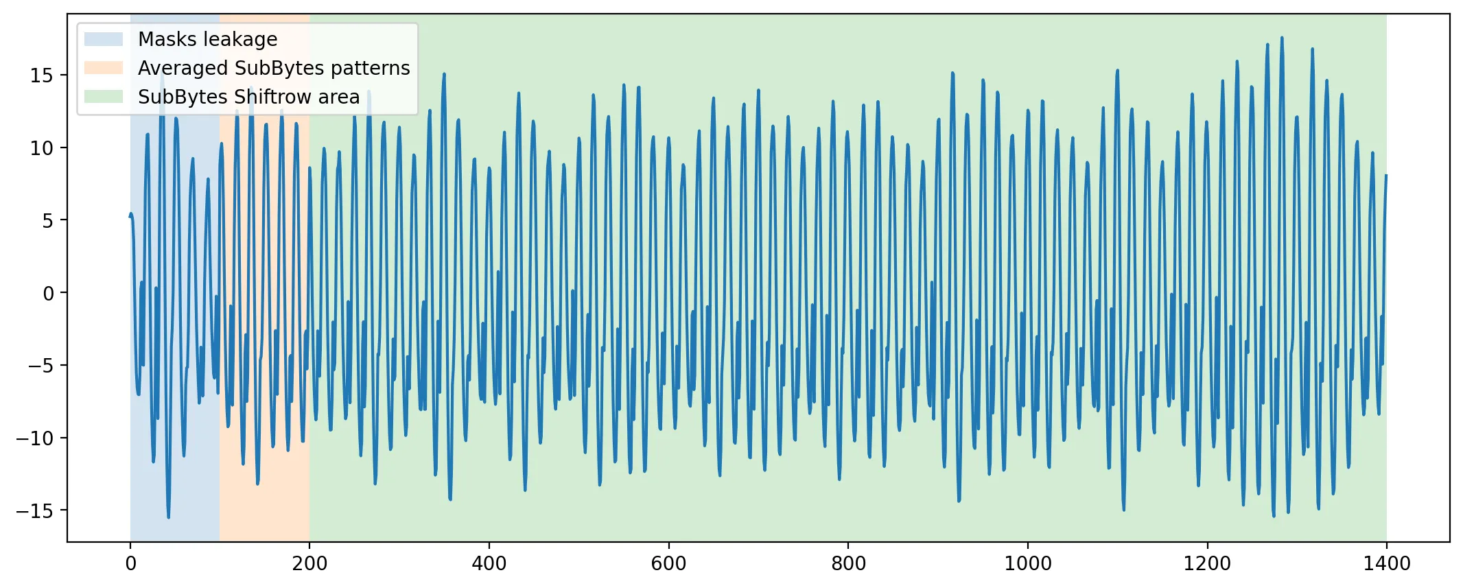
To simplify the analysis, we made the hypothesis that the attacker was able to identify an area of leakage of the mask, which is mandatory for second-order attacks.
In fact, this area was located just before the Sbox table recomputation in our software implementation.

Classical Approach

At first, we are going to unfold an attack using classical tools. As we already made sure that the signal is well aligned, and have identified an area of leakage of the mask Hamming weight, we can then apply a second-order CPA using the centered product.

from estoolkit2.method.sym.analysis import Attack
from estoolkit2 import guessing_entropy as ge


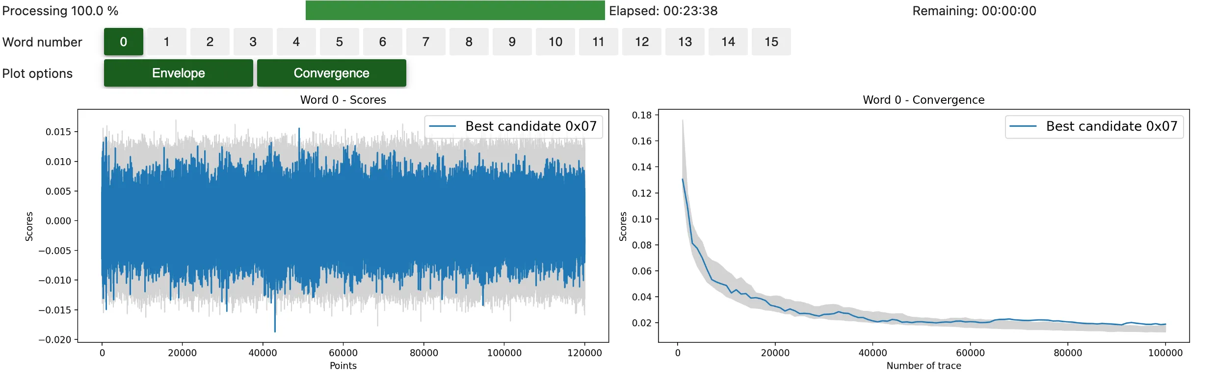
We perform a second-order CPA attack targeting the Hamming weight of the First SubBytes. As high-order recombination function, we use the Centered product. We attack the whole 100,000 traces and compute the convergence score every 1,000 trace.

n_traces, conv_step = 100_000, 1000

attack = Attack(
   ths[:n_traces],
   preprocess=scared.preprocesses.high_order.CenteredProduct(
       frame_1=frames['mask'],
       frame_2=frames['all_SubBytes']),
   selection_function=scared.aes.selection_functions.encrypt.FirstSubBytes(),
   model=scared.HammingWeight(),
   distinguisher=scared.distinguishers.CPADistinguisher(),
   discriminant=scared.discriminants.maxabs,
   n_convergence=conv_step,
)
attack.run()
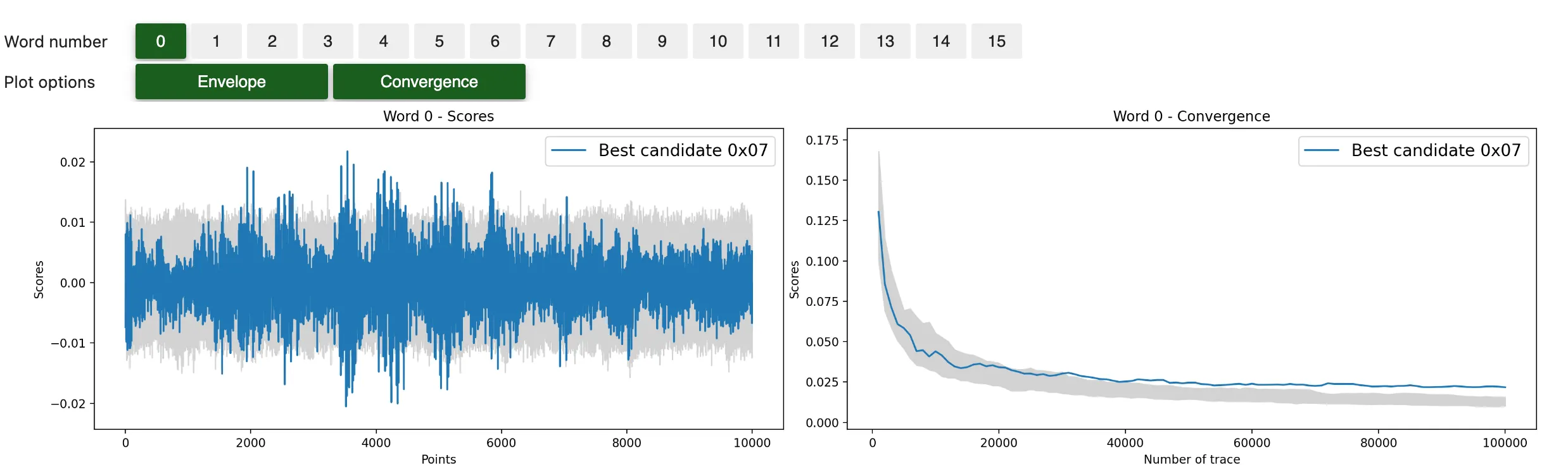
attack.show_result()


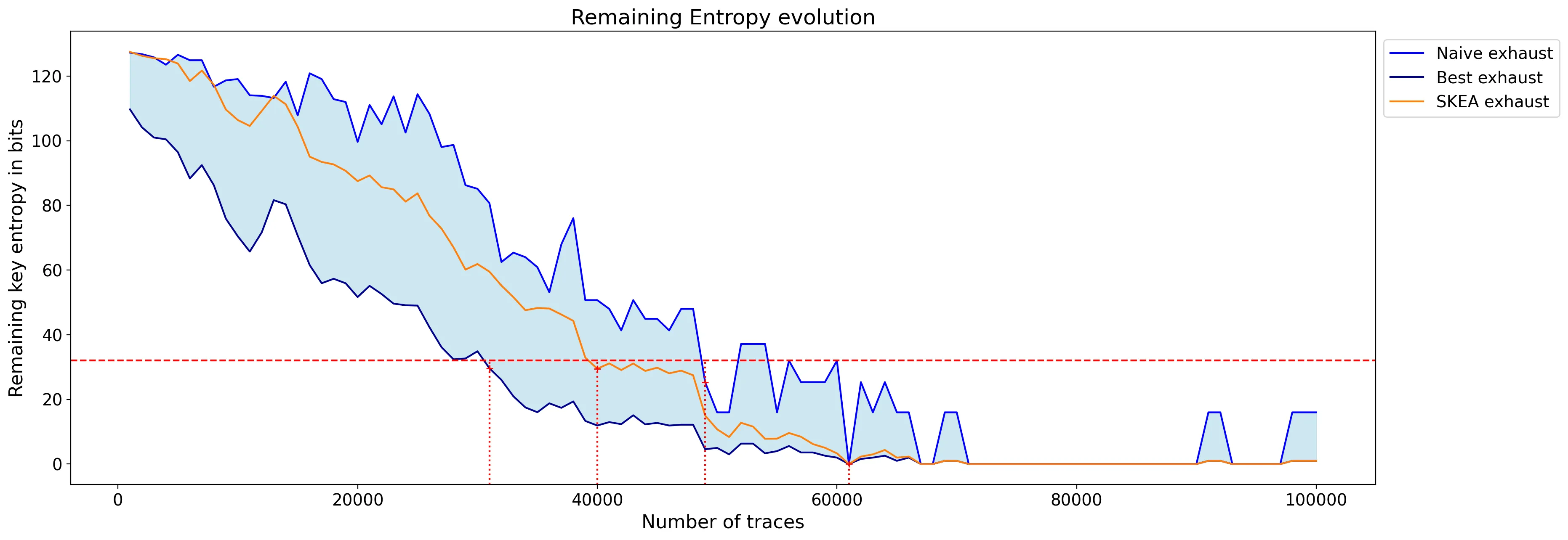
# Compute the remaining guessing entropy
ge.plot_guessing_entropy(ge.guessing_entropy_from_attack(attack))


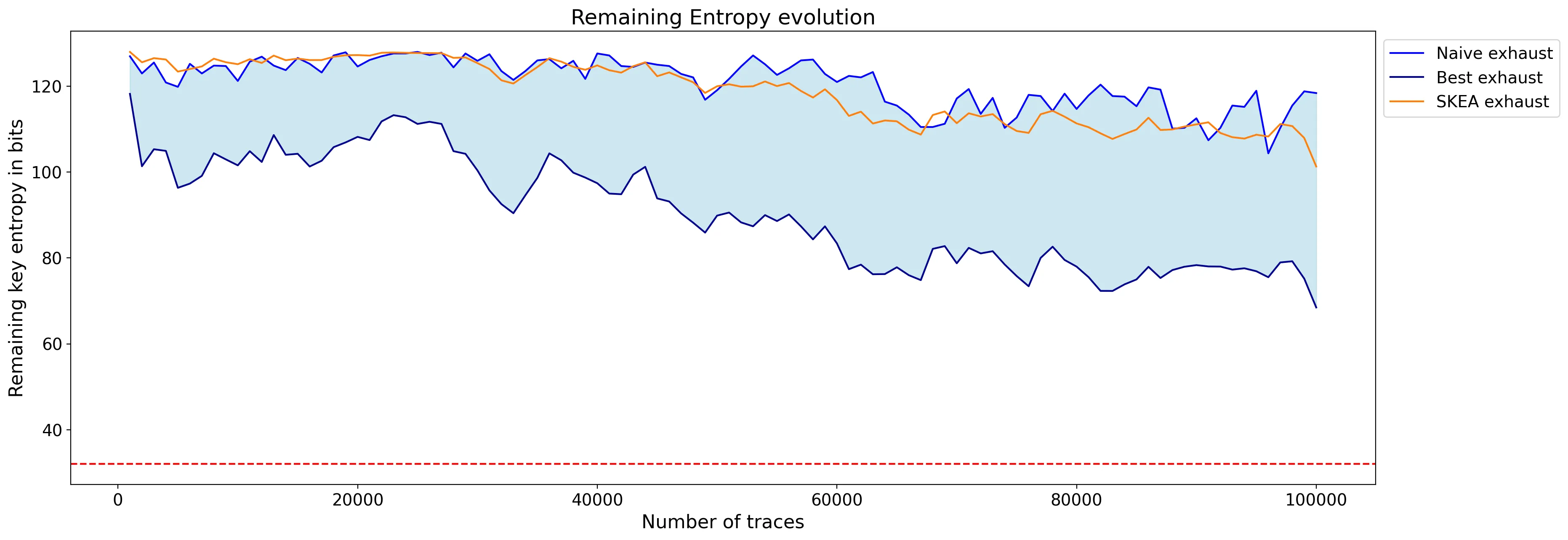
As you can see, the attack does not work using 100,000 traces: the remaining guessing entropy is above 80 and no key byte was found at the end. So the shuffling countermeasure, on top of Boolean masking, is efficient to thwart this straightforward second-order CPA.

The leakage is still present, but hidden in a lot of noise, due to the shuffling countermeasure. In fact, the dataset at the time-index of attack is comprised of 6,250 (or 100,000/16) samples of leakage in average, and 93,750 (or 100,000*15/16) samples of noise, making the attack impractical.

Refining the CPA through PoI averaging

A simple way for the attacker to increase the efficiency of this CPA attack facing shuffling, is to average all SubBytes patterns together. Then it has to use the centered product to combine the mask leakage and the averaged SubBytes leakage. Doing so, it will ensure every trace brings meaningful information to the distinguisher. Yet, this leakage will be the average of 16 samples, which also brings a lot of unnecessary variations to the analysis.

Most importantly, this technique requires fine characterization of the masked SubBytes leakage. Indeed, in order to average the SubBytes patterns together… you must identify them! We let the reader, as an exercise, the freedom to come up with a technique to identify the points of interest without knowledge of the key and masks, in blackbox analysis context.

Using the mask and key knowledge, these area were easily identified (refer to the notebook in gitlab).

n_traces, conv_step = 100_000, 1000

attack = Attack(
   ths[:n_traces],
   preprocess=scared.preprocesses.high_order.CenteredProduct(
       frame_1=frames['mask'],
       frame_2=frames['avg_SubBytes']),
   selection_function=scared.aes.selection_functions.encrypt.FirstSubBytes(),
   model=scared.HammingWeight(),
   distinguisher=scared.distinguishers.CPADistinguisher(),
   discriminant=scared.discriminants.maxabs,
   n_convergence=conv_step,
)
attack.run()
attack.mini_report(verbose=False)
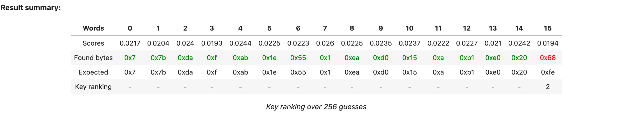
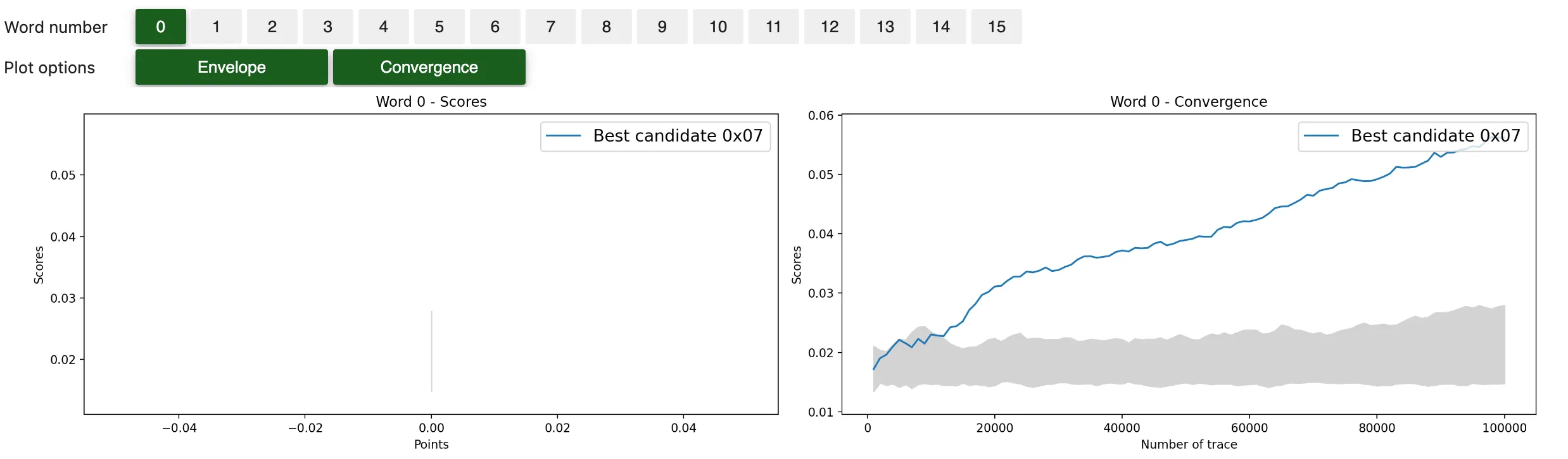
attack.show_result()


Result summary:

ge.plot_guessing_entropy(ge.guessing_entropy_from_attack(attack))


With this technique, all key bytes are recovered with approximately 60,000 traces but some bytes can be subject to noise and are challenged by other key candidates. Even after 100,000 traces, one of the byte is still not ranked first.

Scatter and Spatial Dependency Analysis Approach

Unlike the classical approach, the idea here is to focus on the distribution of the whole trace, and extract leakages from it by leveraging the Spatial Dependency Analysis, and in particular Moran’s Index. The details of an implementation of this attack are described in [1].

So at second-order, we first merge the distribution of all samples in the mask area together with the samples in the SubBytes+ShiftRows area. The joint-distribution are then analyzed using Moran’s Index in order identify the secret key.

import escatter as es
n_traces, conv_step = 100_000, 1000
n_bins = 64
scatter_processing = [es.processing.compute_interaction_information,
                     lambda acc: es.processing.compute_moran(acc, k=7, d=5)]

scatter_distinguisher = es.distinguisher.ScatterSecondOrder(
   processing=scatter_processing,
   scoring=es.scoring.sum_abs,
   frame_1=frames['mask'],
   frame_2=frames['all_SubBytes'],
   histogram_generator=es.histogram.HistogramGenerator(bins_number=n_bins),
   partitions=range(9))

scatter_attack = Attack(
   ths=ths[0:n_traces],
   selection_function=scared.aes.selection_functions.encrypt.FirstSubBytes(),
   model=scared.HammingWeight(),
   distinguisher=scatter_distinguisher,
   discriminant=scared.discriminants.maxabs,
   n_convergence=conv_step)

scatter_attack.run()
scatter_attack.show_result()


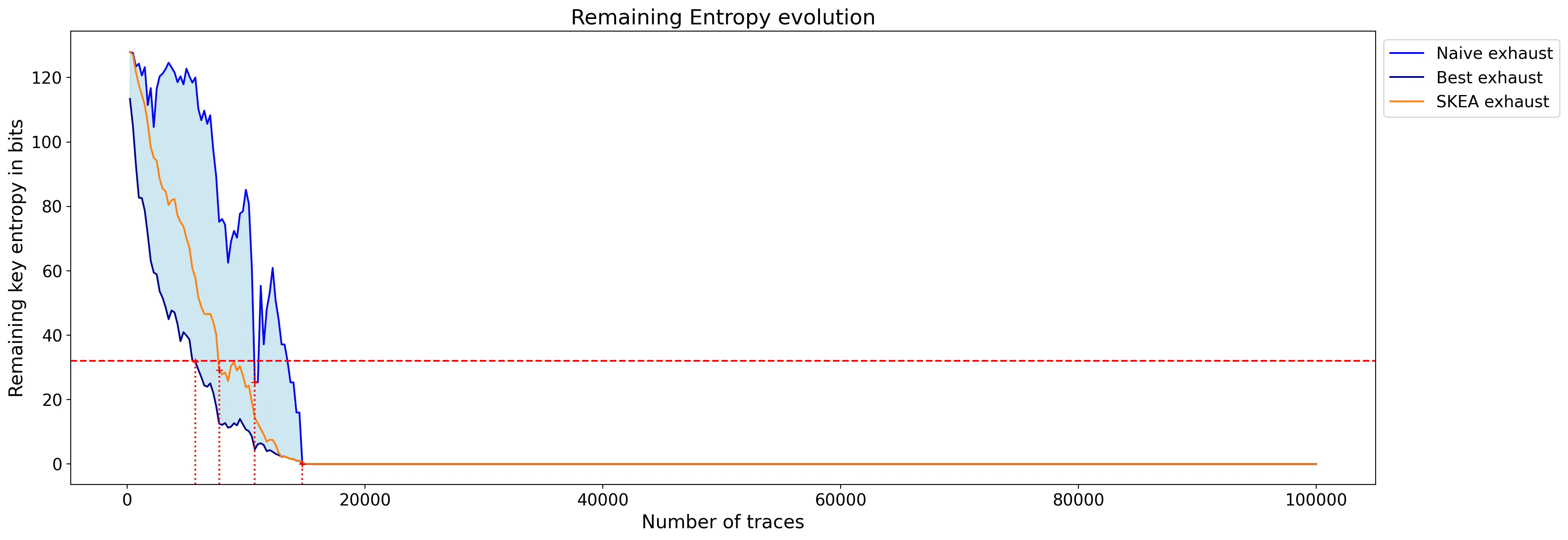
We can see that the attack is much more efficient, despite not requiring to carefully select only points of interest. It could eventually be further refined by selecting points of interest, and also by fine tuning hyper-parameters, such as Moran’s kernel.
Yet, in practice, it is already over: the key is retrieved with only 15,000 traces!

ge.plot_guessing_entropy(ge.guessing_entropy_from_attack(scatter_attack_2))


Conclusion

We developed this technique, leveraging spatial dependency analysis, to tackle difficult and noisy side-channel signals.

In this simple use-case of masked and shuffled AES, even if the microcontroller has strong side-channel leakages, the countermeasures make that classical CPA-based techniques require in the range of 60,000 traces to recover the secret key. After 100,000 traces, it seems that some key bytes attacked are still suffering from noise, and could be hard to distinguish from other candidates. Moreover, this attack requires to precisely identify the clock cycles in which each of the 16 SubBytes computation happens, prior to the knowledge of the secret key; and as you can see in the raw traces, that is not a straightforward task.

In the meantime, when working with the simultaneous distribution of multiple samples, one can roughly select the area of computation of the 16 SubBytes+ShiftRows as a whole, combine that with a distribution containing leakage samples of the mask, and let the spatial distribution analysis extract valuable leakage from this complex mixture distribution. Doing so, the key could be recovered in only 15,000 traces, with clear distinguishability, and without fine characterisation of the points of interest in the trace. It thus appears in this masked and shuffled use case that spatial dependency analysis could be a very practical and efficient tool to extract information from intricate side-channel traces.

References

[1] Vasselle, A., Thiebeauld, H. & Maurine, P. - Spatial dependency analysis to extract information from side-channel mixtures: extended version. - Journal of Cryptographic Engineering (2023). - https://doi.org/10.1007/s13389-022-00307-9

‍