Ledger Donjon CTF Fine Fine write-up

We hooked an oscilloscope to a chip we found on the floor near the entrance of the Crypto-Party. It executes what looks like the public key computation on secp256r1 from some static secret, but it seems we can specify the input point though… And it’s definitely a Montgomery Ladder. That secret in there must give us access to free cryptodrinks, surely?

Introduction

To be fair, I did not find the right attack path so quickly. I tried a lot of techniques like cross correlation, or trying to find some bit values as I know that the scalar contains “CTF{”. But without success. After a discussion with my colleague Pierre-Yvan Liardet about the possible attack paths against:

a scalar multiplication
using Montgomery ladder
with point randomization
knowing that I can choose the point to multiply

he pointed me directly to an attack from Louis Goubin [Goubin2003] so called the “Refined attack”, a chosen point attack. Mais oui mais c’est bien sûr! Fine fine -> Refined -> correct attack!

I’m sure that I’m on the right track! Let’s implement it.

Attack theory

The refined attack is a chosen point method to attack scalar multiplication. It is compatible with Montgomery ladder, projection and point randomization.

The main idea is to obtain, at some step of the calculus a point $P^$ with a null coordinate. If the implementation is not sufficiently robust, the operations involving $P^$ should have a different signal. Indeed, regardless of the formulas used to perform the addition or the doubling, they will involve a lot of calculus with zero values, that can lead to differences in the power consumption compared to non-zero values.

First, a quick reminder about the Montgomery ladder algorithm. In the following, the registers $R_0$ and $R_1$ usually found in the literature are replaced by $A$ and $B$ to avoid double indexing.
Let $(d_m, …, d_0)$ the binary form of the scalar $d$. The Montgomery ladder algorithm to perform the multiplication of the point $P$ by $d$ is the following:

A ← 0 B ← P for i from m downto 0 do if d_i = 0 then B ← point_add(A, B) A ← point_double(A) else A ← point_add(A, B) B ← point_double(B) return A

If we are looking at the operand of the double and add operations, we can see that:

the add operation always performs $A + B$, regardless of the value of $d_i$
depending on the value of the bit $d_i$, the double operation is performed either on $A$ if $d_i$ is 0 or on $B$ if $d_i$ is 1.

And knowing the bits $(d_m, …, d_{i-1})$ we can build a special point $P^$ such as $A$ or $B$ equal $P^$ when $d_i$ is processed. And then the second observation can be used to distinguish bit values.

Compute (precursor of) special point $P^*$

We want to find a point $P^*$ with a null $x$ coordinate.

The challenge uses the secp256r1 elliptic curve (we will use the tinyec package to work with this curve). As the curve equation is $y^2=x3 + ax + b$, a point $P^* = (0, \\sqrt b)$ is on the curve and should do the job. Then let’s compute $\\sqrt b$ (how to calculate modular square roots).

First, we need to check that $b$ is a quadratic residue modulo the prime $p$:

from tinyec.registry import get_curve curve = get_curve('secp256r1') p = curve.field.p pow(curve.b, (p - 1) // 2, p) 1

Yes it is!
The method to compute the square root depends on the modulo:

print('p congruent to 3 mod 4: ', p % 4 == 3) print('p congruent to 5 mod 8: ', p % 8 == 5) print('p congruent to 1 mod 8: ', p % 8 == 1) p congruent to 3 mod 4: True p congruent to 5 mod 8: False p congruent to 1 mod 8: False

We are in the easy case $p\equiv 3\mod 4$! The square roots of $b$ can be computed as $r \equiv \pm b^{(p + 1) / 4} \pmod p$

root = pow(curve.b, (p + 1) // 4, p) assert pow(root, 2, p) == curve.b root 46263761741508638697010950048709651021688891777877937875096931459006746039284

Let’s now define the point $P^* = (0, \\sqrt b)$:

from tinyec import ec p_star = ec.Point(curve, 0, root) p_star (0, 46263761741508638697010950048709651021688891777877937875096931459006746039284) on "secp256r1" => y^2 = x^3 + 115792089210356248762697446949407573530086143415290314195533631308867097853948x + 41058363725152142129326129780047268409114441015993725554835256314039467401291 (mod 115792089210356248762697446949407573530086143415290314195533631308867097853951)

But it is not sufficient to perform the attack. We want a “precursor” of $P^$, i.e. a point $P’$ such as for a given scalar $k$, $k \cdot P’ = P^$. This point $P’$ is easy to find: $P’ = (k^{-1} \mod n ) \cdot P^*$, where $n$ is the group order.

We can define a function to compute $P’$ for a given scalar:

def generate_p_prime(scalar): """Generate a point P' such as known_scalar x P = P*""" curve = get_curve('secp256r1') p = curve.field.p root = pow(curve.b, (p + 1) // 4, p) p_star = ec.Point(curve, 0, root) inv = ec.mod_inv(scalar, curve.field.n) p_prime = inv * p_star assert (scalar * p_prime).x == 0 return p_prime # Check that we get p_start (having x==0) with k=3 p_prime = generate_p_prime(3) 3 * p_prime (0, 46263761741508638697010950048709651021688891777877937875096931459006746039284) on "secp256r1" => y^2 = x^3 + 115792089210356248762697446949407573530086143415290314195533631308867097853948x + 41058363725152142129326129780047268409114441015993725554835256314039467401291 (mod 115792089210356248762697446949407573530086143415290314195533631308867097853951)

Observe the traces

It is now time to observe the traces. The challenge comes with a client.py file which provides a function send_getpubkey that asks the chip to perform the scalar multiplication for a given point and then return the recorded power trace. As a reminder, the goal is to find the secret scalar k used by the chip to perform point multiplication.

Let’s try it with the curve base point $G$ (twice):

point2str = lambda point: point.x.to_bytes(32, byteorder='big').hex() + point.y.to_bytes(32, byteorder='big').hex() from client import send_getpubkey base_trace = send_getpubkey(point2str(curve.g)) base_trace_2 = send_getpubkey(point2str(curve.g)) import matplotlib.pyplot as plt plt.style.use('./matplotlib.style') plt.plot(base_trace) plt.plot(base_trace_2) plt.xlim(10_000, 11_000) plt.title('Zoom on returned traces for scalar mult on G') plt.show()

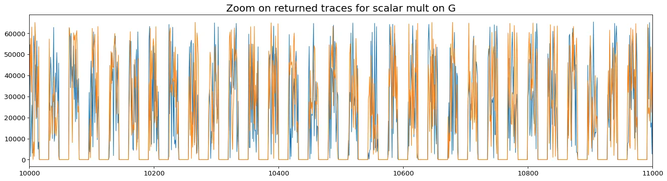
The trace is composed of 11,506 patterns separated by a sequence of zero values. And we can see that the two traces are different even if we requested the same point computation. This indicates the presence of the point randomization countermeasure, which is almost free when projective coordinates are used.

We can now observe what is happening when the point $P’_2$ (resp $P’_3, ~~P’_4, …$), i.e. the point such as $2 \cdot P’_2 = P^$ (resp $3 \cdot P’_3 = P^, ~~4 \cdot P’_4 = P^*, …$ is processed.

import numpy as np traces = [] for scalar in range(2, 6): traces.append(send_getpubkey(point2str(generate_p_prime(scalar)))) traces = np.vstack(traces)

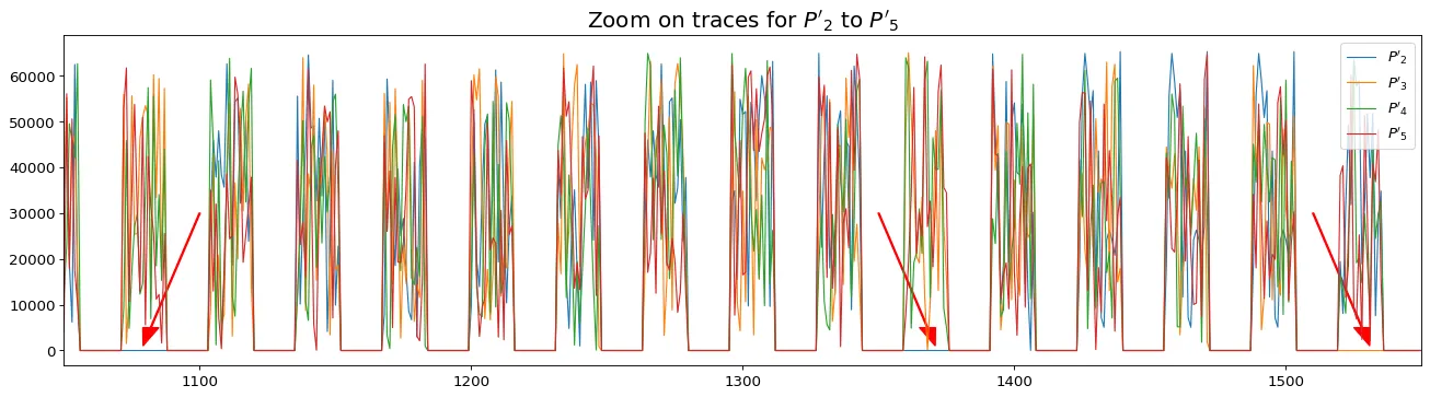
As shown with red arrows in the following figure, we can observe some new zero values obtained with $P’_k$ for different $k$ values.

plt.plot(traces.T[:2000]) plt.xlim(1050, 1550) plt.legend(labels=[f"$P'_{i}$" for i in range(2, 6)]) plt.title("Zoom on traces for $P'_2$ to $P'_5$") plt.arrow(1100, 30000, -18, -25000, color='red', width=0.5, head_width=6, head_length=4000) plt.arrow(1350, 30000, 18, -25000, color='red', width=0.5, head_width=6, head_length=4000) plt.arrow(1510, 30000, 18, -25000, color='red', width=0.5, head_width=6, head_length=4000) plt.show()

Attack the traces

These zero values can be used to decide if the bit $d_i$ is 0 or 1 with the following methodology:

Let $d^j$ the $j$ known first bits of the scalar $d$. During the $(j + 1)$-th iteration of the scalar multiplication of $P$, we have $A = d^j \cdot P$ and $B = (d^j + 1)\cdot P$. And then, as explained previously, the double operation is performed on either $d^j \cdot P$ or $(d^j + 1)\cdot P$ depending on the current bit value.

To make $P^*$ appear at iteration $j+1$, in either $A$ or $B$, we can generate the traces for both $P’{d^j}$ and $P’{d^j + 1}$. By observing which one has the higher number of zero values, we will distinguish if the double operation is performed on $A$ or $B$ and then obtain the current bit value. To improve the process efficiency, we can use averaged traces.

The following function takes a known scalar as input and then returns the current bit processed is or 1:

def find_bit(known_scalar): n = 2 mean_a = np.mean([send_getpubkey(point2str(generate_p_prime(known_scalar))) for _ in range(n)], 0) mean_b = np.mean([send_getpubkey(point2str(generate_p_prime(known_scalar + 1))) for _ in range(n)], 0) return int((mean_a == 0).sum() < (mean_b == 0).sum())

We can now automate the process to retrieve each of the 256 bits. To start, we can consider that the first bit is 1 and the process bit by bit:

from tqdm.notebook import tqdm d = '1' for _ in tqdm(range(255)): di = find_bit(int(d, 2)) d += str(di) d 0%| | 0/255 [00:00<?, ?it/s] '1011100010010111010101000100101110001100011101011100001110010101101100110100001101010100010001100111101101000111011010000110111101110011011101000111001101011111011000010110111001100100010111110100011101101111011101010110001001101001011011100111001101111101' int(d, 2).to_bytes(length=32, byteorder='big') b'\xb8\x97TK\x8cu\xc3\x95\xb3CTF{Ghosts_and_Goubins}'

It works! The flag is CTF{Ghosts_and_Goubins}.

Thanks

… to the Ledger Donjon team to provide the community with this CTF. I have to confess that it is the first time I put into practice the refined Goubin attack. Thanks to improve my side-channel skills and more generally to contribute to a better global hardware security.

References

[Goubin2003] Louis Goubin. (2003). A Refined Power-Analysis Attack on Elliptic Curve Cryptosystems. link

‍