The Challenge

Lately I have been using AI intensively mostly for reverse engineering and software development through the esDynamic and esReverse platform. I have not done much side-channel analysis for the past years and wanted to see how AI could help there (TL-DR a lot!). I was already convinced that being assisted by AI is already a must, but to convince other experts you often have to prove it on real case study. As my father-in-law often says "You can’t teach experience"

‍I had in mind this dataset published by eShard previously — an STM32F446 running AES-128 with first-order boolean masking and SubBytes shuffling — I wondered: could I use esDynamic platform with its AI solution as a research partner to replicate, understand, and improve the published attack in a single afternoon and see how far I can go. I only used public information, nothing coming from internal work or our internal RAG.

The target is genuinely hard. The implementation combines two protections:

• Boolean masking: the SBOX output is XOR’d with a random mask — perfect leakage = HW(SBOX[pt ⊕ k] ⊕ mask). Without knowing the mask, direct correlation fails.
• SubBytes shuffling: the 16-byte operations execute in a uniformly random order per trace. Even if you defeat the masking, you don’t know which time slot carries the leakage for which byte.

The corresponding paper (Spatial dependency analysis, ASHES@CCS 2021) proposes the Scatter + Moran attack. It combines different statistical tools to achieve a second order attack. My goal: replicate it, then try to improve it in a short window of time.

‍

Results

Starting from a zero SCA context (public paper and dataset), a pair-programming session with a LLM produced:

• A working paper replication in 1 hour
• Genuine improvement through wavelets:
  • 33% improvement over the proposed attack (in traces number)
  • 2.5x MIA improvement in the number of traces required to recover the secret key. (50k → 20k)
• A complete Rust implementation running in 2.5 seconds
• A systematic exploration of histogram alternatives (all negative, but informative)
• A reusable simulation framework for discriminant benchmarking

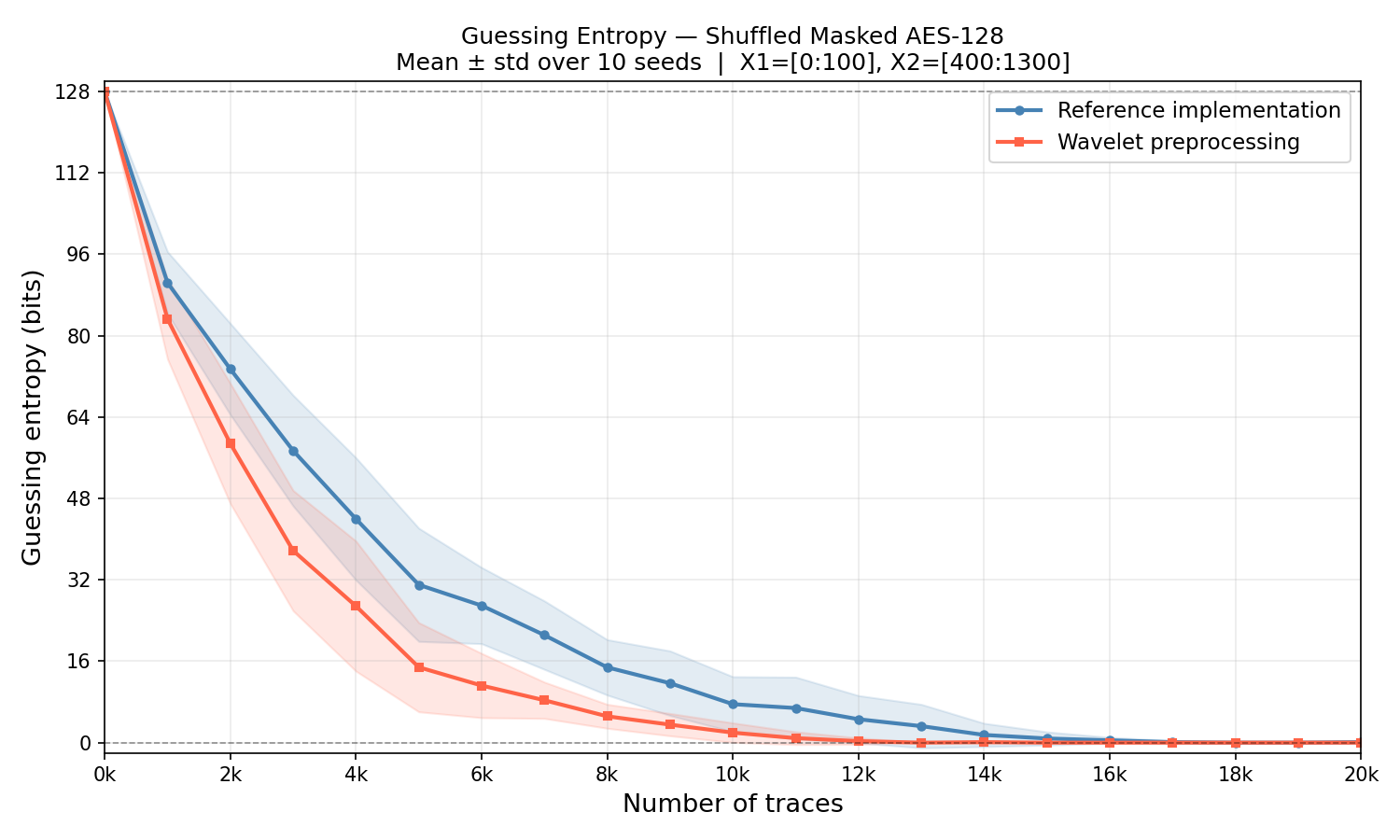
The paper achieves 16/16@15k (16 bytes of the secret AES128 key out of 16 with 15k traces) as “best of 10 seeds” — their lucky seed. We achieve 16/16@15k on all 10 seeds. That’s a stronger result under a harder criterion. At 10k traces, wavelet already succeeds on 80% of seeds vs the paper’s 0%.

Timeline

‍

Total LLM + script running time: ~24 hours of compute, ~half a day of my attention.

Implications: If, as me, you would need more than half a day to read, understand, implement and try new ideas to improve this paper, then it’s probably worth using an AI platform designed for side channel.

‍

Thoughts on IA

While headlines often oscillate between AI being an all-powerful replacement for humanity or a digital Pandora’s box too dangerous to open, the reality is far more practical.

AI isn’t a substitute for human intelligence, but a multiplicative factor. It functions as a high-speed engine that allows you to iterate rapidly and scale your productivity. However, just like a ship needs a captain, the expert remains essential to provide direction, navigate complexity, and move beyond the mediocre. It is, quite simply, a premier tool for those who know how to steer it.

Why the expert is still necessary?

• Intuition: Understanding the “why” behind a project, including office politics, market sentiment, and long-term vision.
• Accountability: A model cannot be held liable for a bridge collapsing or a medical misdiagnosis. Humans must remain in the loop to carry the moral and legal weight of decisions.
• “Last Mile” Problem: AI can often get you 80% of the way much quicker. However, that final 20%—the nuance, the creative edge, the factual verification—requires human judgment.

We aren’t moving toward a world where AI replaces the doctor, the lawyer, or the engineer. From my perspective as of today, we are moving toward a world where the expert using AI replaces the expert who doesn’t.

‍

The Technical part

The Attack Pipeline

Before diving into improvements, here’s what the paper’s scatter+Moran attack does.

Every trace is split into two windows:

• X1 = samples[0:100]: the mask leakage window. The mask XOR creates a power signature correlated with HW(mask).
• X2 = samples[400:1300]: 900 samples covering all 16 SubBytes operations (in shuffled order).

The scatter histogram is the key idea: instead of looking at specific time positions (which change trace-to-trace due to shuffling), build a 2D amplitude histogram of (X1_amplitude, X2_amplitude) pairs across all 100×900 = 90,000 sample pairs per trace:

T[i, b1, b2] = count_x1[i, b1] × count_x2[i, b2]


This outer product is shuffle-invariant — it doesn’t matter which time slot each byte occupies. The correct key creates a coherent blob in (b1, b2) space because the mask constrains both windows simultaneously. Moran’s spatial autocorrelation index detects this blob.

‍

Replication

Within the first hour, the LLM had produced a working Python implementation matching Table 1 of the paper:

Scatter + Δ_I + Moran, NB=32, X2=[400:1300] → 16/16 keys at N=15k (single seed)


This is the paper’s “No Averaging” result. The implementation:

1. Build T_flat using fast one-hot GEMM (build_histograms_fast)
2. Compute the Δ_I differential field (Spatial dependency analysis Eq. 12)
3. Score with Moran’s I box-filter (7,7,5)

‍

Improvement 1: Performances

During the analysis I found that Δ_cov and Δ_I produce empirically identical Moran scores.

The covariance-based differential field Δ_cov(H_correct, H_marginal) produces bit-for-bit identical Moran scores to the Δ_I formulation from the paper when both fields are subsequently passed through Moran’s spatial filter — and is computationally cheaper, since Δ_cov avoids the per-cell log computation and reduces to a single matrix subtraction. All Moran-based results in this post use Δ_cov.

Note on equivalence: this is empirical equivalence under Moran scoring, not algebraic identity. Δ_I = P·log(P/Q) and Δ_cov = P−Q are nonlinearly related; Moran’s spatial averaging absorbs the linearisation error in practice. The equivalence does not extend to MIA-style summation without Moran — see Improvement 2 below.

‍

Improvement 2: Wavelet Preprocessing

I tried different distinguishers and preprocessing to improve the attack on the provided traces and found quickly that wavelet was quite an improvement !

What the wavelet does

The raw X2 window contains 900 samples of mixed signal: DC power supply drift, clock oscillations, SubBytes leakage pulses (~56 samples per byte operation), and noise. Most of this is irrelevant.

We approximate the SWT db4 level-3 detail with a cheap single-stage filter: the upsampled db4 high-pass hu = h↑4 applied directly to X2. This is not a true SWT (we skip the level-1/2 low-pass cascade), so hu has spectral replicas at fs/16, 3fs/16, 5fs/16, 7fs/16 — but the SubBytes leakage band sits squarely on the main lobe at fs/16 ≈ 12.5 MHz, so the approximation works in practice.

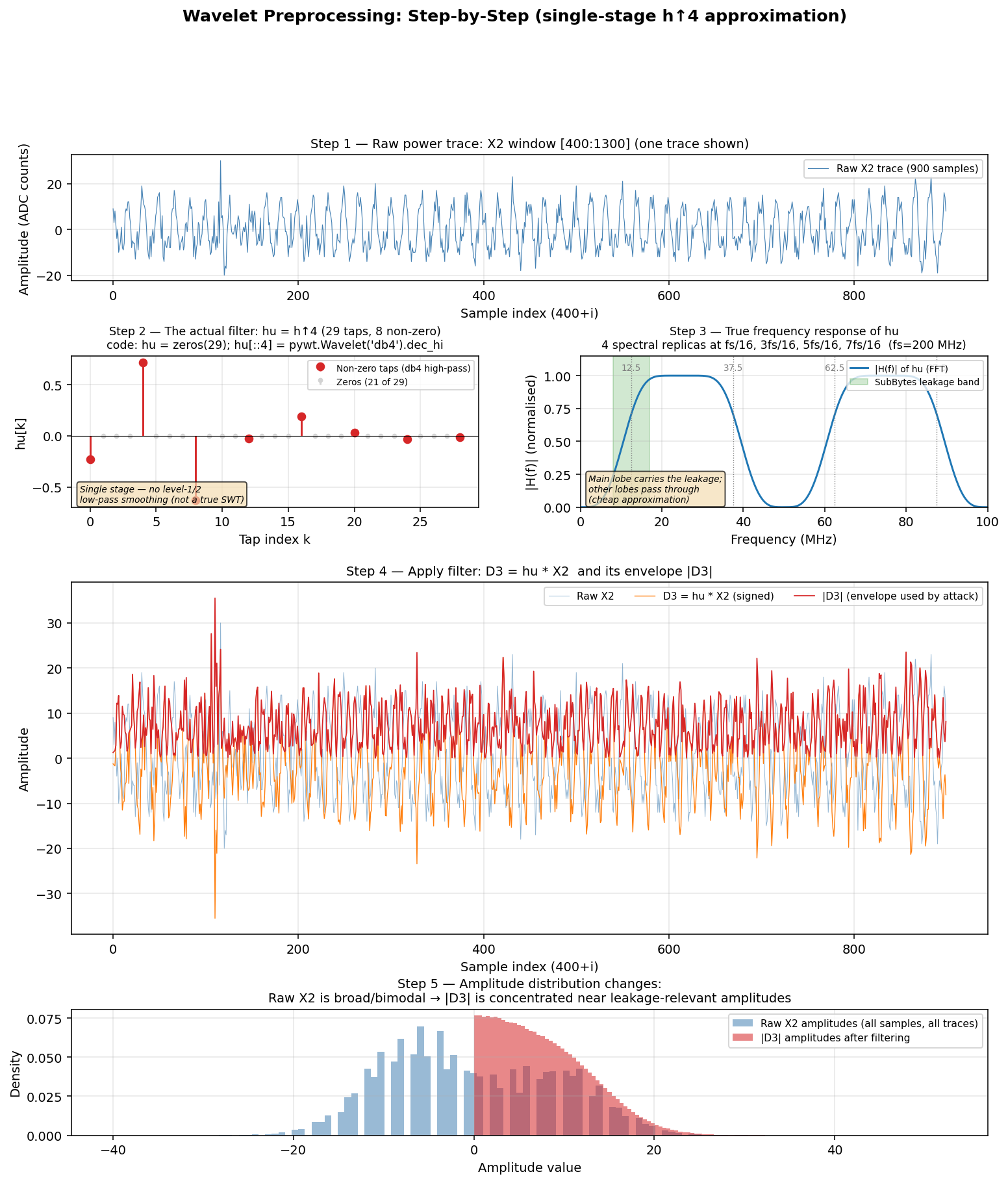
The computation is simple — a 29-tap convolution followed by absolute value:

h  = np.array(pywt.Wavelet('db4').dec_hi)
hu = np.zeros(len(h)*4 - 3)
hu[::4] = h                          # upsample by 4 (level 3)
X2_wavelet = np.abs(convolve1d(X2, hu, axis=1, mode='reflect'))

Each point D3[n] is simply a weighted sum of 8 samples spaced 4 apart:

D3[n] = h[0]·X2[n] + h[1]·X2[n-4] + h[2]·X2[n-8] + ... + h[7]·X2[n-28]

The blob in (b1, b2) amplitude space becomes sharper and better separated between HW classes. Moran detects it with less data.

‍

Results

Replacing raw X2 amplitudes with |D3| wavelet coefficients reduces the required trace count by 33%:

The guessing entropy curve shows the advantage clearly across 10 random seeds (see first guessing entropy graph, NB = number of bins used)

‍

MIA also benefits from wavelet

Beyond scatter-based scoring, we also tried to improve MIA (Mutual Information Analysis)

Important: the formula must use Δ_I, not Δ_cov. sum(Δ_cov) is identically zero for every key hypothesis.

This means sum(Δ_cov) carries zero discriminating information and recovers 0/16 at every trace count up to 50k. The log in Δ_I is load-bearing for MIA: it converts a zero-sum field into a positive-definite divergence. This is the canonical case where Δ_cov cannot replace Δ_I (unlike Moran-based scoring, where the spatial averaging absorbs the difference).

The wavelet preprocessing helps MIA the same way it helps Moran: cleaner amplitude distributions mean a stronger, lower-variance KL estimate.

A 2.5× reduction purely from the wavelet preprocessing — no change to the statistical framework, no Moran spatial filter.

‍

Performance: Python vs Rust

The attack is fast enough in Python (5–10 seconds at N=15k), but we implemented a Rust version using the faer library for GEMM acceleration and Rayon for parallelism. Build and run with:

cd wavelet_attack_rust && cargo build --release
./target/release/wavelet_attack --nb 16 --cov

The Rust NB=16 config is the recommended production setting: 2.5 seconds for full key recovery at N=15k, parallelized across all available CPU cores via Rayon.

Night Session: Exploring Histogram Alternatives and New Discriminants

With the scatter pipeline thoroughly optimized, a systematic exploration ran overnight (zero manual interactions just implement a big plan and let it run).

Histogram alternatives

The question: can we replace the uniform-bin histogram with something better?

“Scatter” is defined as the uniform-width binning step (digitize_uniform). Any other binning or projection counts as “non-scatter”. We tested six alternatives (the last two rows are variants of the scatter baseline included for comparison):

Three lessons emerged:

1. Binary integer sparsity is essential — soft/fractional bins destroy the signal
2. Absolute amplitude scale must be preserved — quantile normalisation erases the blob
3. All 90k pairs contribute equally — subsampling always degrades ∝√(pairs removed)

R1-pc: a new discriminant

Alongside histogram alternatives, we explored R1-pc: apply a Gaussian post-convolution to the Δ_cov field before computing Moran’s I, rather than using the raw Δ_cov values. Formally:

score_R1pc[g] = Moran_I( G_{σ₁,σ₂} * Δ_cov(H_g, H_m) )

where G_{0.7, 1.5} is a 2D Gaussian kernel with σ_b1=0.7, σ_b2=1.5 applied independently on the two histogram axes (implemented as gaussian_filter(Δ_cov_field, sigma=[0.7, 1.5, 0])), and * denotes 2D convolution over the (NB × NB) amplitude plane. The depth axis (HW classes) is left unsmoothed.

This sub-bin-width smoothing reduces quantisation noise in the Moran estimator without smearing the coherent HW blob. On raw X2, R1-pc is consistently +1–3 bytes over plain Scatter+Moran at small N. However, once wavelet preprocessing is applied, R1-pc’s advantage disappears — the wavelet already delivers a clean high-SNR blob, and the additional Gaussian blur over-smooths it. R1-pc’s real value only became clear in the simulation study (see below), where it proved the most robust discriminant at high noise levels.

‍

Simulation Framework

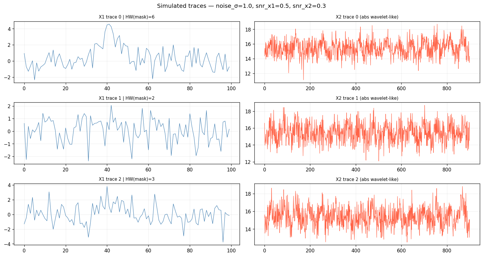
To systematically compare discriminants across different noise conditions, I built a simulation framework that generates synthetic masked+shuffled AES traces, you can see the prototype there and also few simulated sample. We have good traces for the real case, but beeing able to test dynamically could be even nicer.

sim = MaskedShuffledAESSimulator(
    noise_sigma           = 1.0,    # noise level — the main parameter
    snr_x1                = 0.5,    # mask leakage strength in X1
    snr_x2                = 0.3,    # SubBytes leakage strength in X2
    n_x1_leaking          = 20,     # X1 samples carrying mask leakage
    n_x2_leaking_per_slot = 8,      # samples leaking per byte slot (of 56)
    apply_abs             = True,   # return |X2| to mimic wavelet envelope
)
X1, X2, plaintexts, masks, key = sim.generate(N=10000)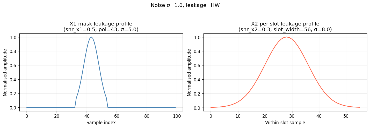

‍

Discriminant comparison across noise levels

9 discriminants tested at 8 noise levels (σ=0 to 3.0), N=5000 traces each:

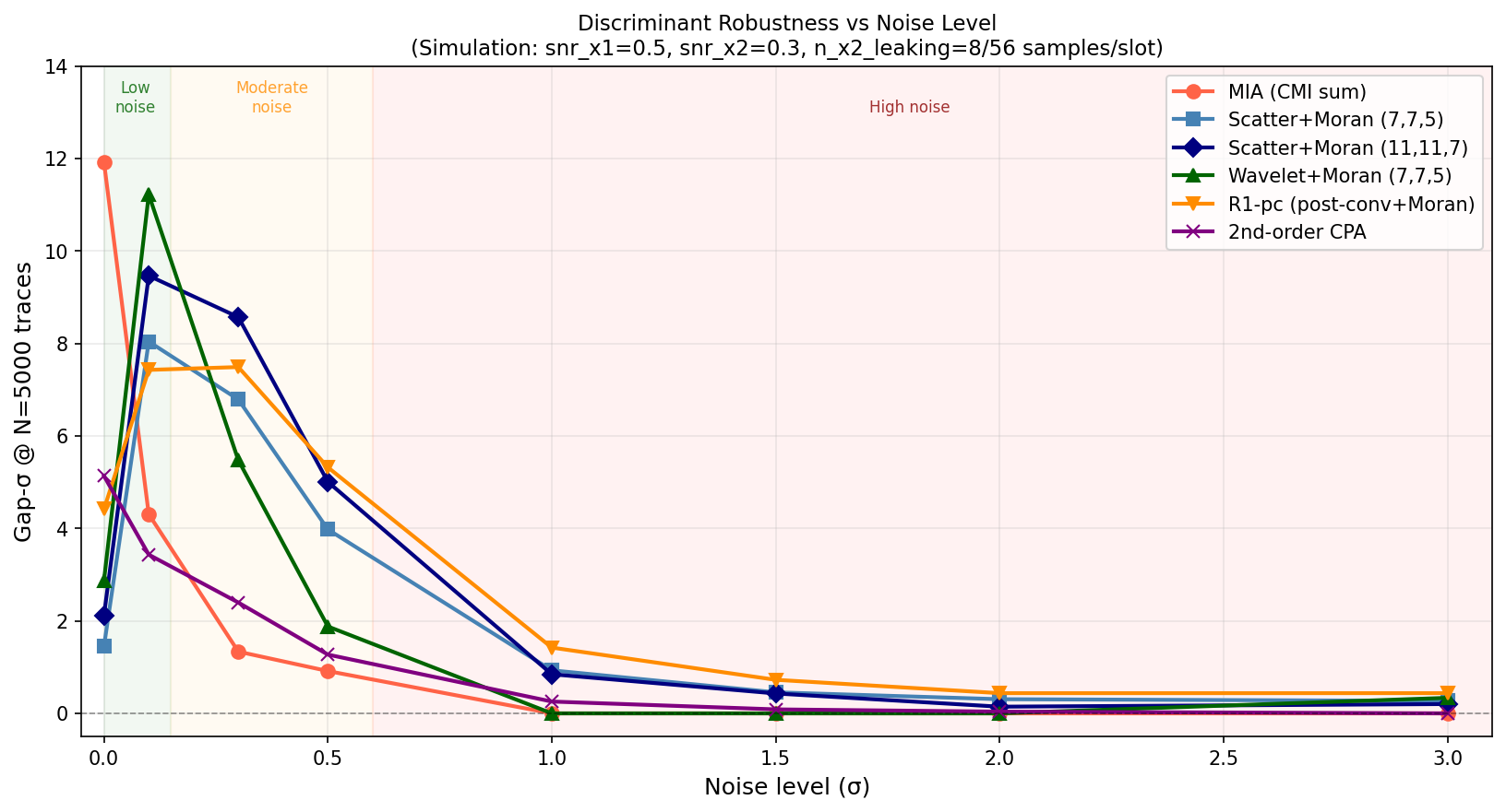
Three noise regimes:

• Low noise (σ≤0.1): MIA wins at σ=0 (no noise, no Moran needed). Wavelet+Moran is best at σ=0.1.
• Moderate noise (σ=0.3–0.5): Scatter+Moran(11,11,7) dominates — larger kernel accumulates coherent blob signal.
• High noise (σ≥1.0): R1-pc is the most robust — maintains signal at σ=2.0 where everything else fails.

The L2 scorer is universally zero — confirming that Moran’s spatial coherence detection is essential, not optional.

‍

Key Contributions Summary

‍

Conclusion

The uniform-bin scatter outer product seems near-optimal under the shuffle-invariant constraint. Six different histogram alternatives all performed worse than the scatter baseline. The “scatter” design, the binary integer sparsity, absolute amplitude scale, and full pair count are all load-bearing.

The wavelet preprocessing is the real contribution: it’s a one-line change (np.abs(convolve1d(X2, upsampled_filter))) that makes the attack 33% more sample-efficient by isolating the SubBytes leakage frequency band from carrier noise and DC drift.

With this investigation, I wanted to explore how efficient AI can quickly digest a paper and provide technical results. For a technique like Scatter, considered too complex to run in comparison to CPA, it was almost trivial to get it working. And I was pleased that it was possible to push the investigations further, by trying many other techniques and finding valuable results. And unlike the apocalypse described by marketing from OpenAI or Anthropic, I definitely confirm the need of a human in the loop.

‍